Excel Create Pareto From Pivot Table - Once your data is sorted and the cumulative percentage is calculated, you can create a pareto chart by. On the insert tab, in the charts group,. Set up your data as shown below. Here are the steps to create a pareto chart in excel: In this article, we'll walk through the process of transforming a pivot table into a pareto chart. To create a pareto chart, start by making a pivot table from your data range. Select the entire data set (a1:c10), go to. Select any data from your dataset. We'll explore why you'd want to use a. To create a pareto chart in excel 2016 or later, execute the following steps.
To create a pareto chart in excel 2016 or later, execute the following steps. To create a pareto chart, start by making a pivot table from your data range. We'll explore why you'd want to use a. Select the entire data set (a1:c10), go to. Select any data from your dataset. Set up your data as shown below. On the insert tab, in the charts group,. Here are the steps to create a pareto chart in excel: In this article, we'll walk through the process of transforming a pivot table into a pareto chart. Once your data is sorted and the cumulative percentage is calculated, you can create a pareto chart by.
To create a pareto chart in excel 2016 or later, execute the following steps. We'll explore why you'd want to use a. To create a pareto chart, start by making a pivot table from your data range. Here are the steps to create a pareto chart in excel: Select the entire data set (a1:c10), go to. Select any data from your dataset. Set up your data as shown below. On the insert tab, in the charts group,. Once your data is sorted and the cumulative percentage is calculated, you can create a pareto chart by. In this article, we'll walk through the process of transforming a pivot table into a pareto chart.
How to Make a Pareto Chart Using Pivot Tables in Excel
On the insert tab, in the charts group,. In this article, we'll walk through the process of transforming a pivot table into a pareto chart. Set up your data as shown below. To create a pareto chart in excel 2016 or later, execute the following steps. Once your data is sorted and the cumulative percentage is calculated, you can create.

Pareto chart in Excel how to create it
To create a pareto chart, start by making a pivot table from your data range. Set up your data as shown below. Select the entire data set (a1:c10), go to. Select any data from your dataset. Once your data is sorted and the cumulative percentage is calculated, you can create a pareto chart by.
Create A Pareto Chart From Pivot Table How To Create A Pareto Chart
We'll explore why you'd want to use a. To create a pareto chart, start by making a pivot table from your data range. Select the entire data set (a1:c10), go to. Set up your data as shown below. Here are the steps to create a pareto chart in excel:

How to Make a Pareto Chart Using Pivot Tables in Excel
In this article, we'll walk through the process of transforming a pivot table into a pareto chart. To create a pareto chart in excel 2016 or later, execute the following steps. We'll explore why you'd want to use a. To create a pareto chart, start by making a pivot table from your data range. Set up your data as shown.

Pareto Chart Excel Pivot Table Pareto Chart With Excel Pivot Table Charts
In this article, we'll walk through the process of transforming a pivot table into a pareto chart. Set up your data as shown below. Select the entire data set (a1:c10), go to. On the insert tab, in the charts group,. We'll explore why you'd want to use a.
How to Make a Pareto Chart Using Pivot Tables in Excel
In this article, we'll walk through the process of transforming a pivot table into a pareto chart. To create a pareto chart, start by making a pivot table from your data range. On the insert tab, in the charts group,. Set up your data as shown below. Select any data from your dataset.

How to Make a Pareto Chart Using Pivot Tables in Excel
To create a pareto chart, start by making a pivot table from your data range. Select the entire data set (a1:c10), go to. Here are the steps to create a pareto chart in excel: Set up your data as shown below. We'll explore why you'd want to use a.
How to Make a Pareto Chart Using Pivot Tables in Excel
In this article, we'll walk through the process of transforming a pivot table into a pareto chart. Here are the steps to create a pareto chart in excel: To create a pareto chart, start by making a pivot table from your data range. On the insert tab, in the charts group,. Once your data is sorted and the cumulative percentage.

How to Make a Pareto Chart Using Pivot Tables in Excel
Here are the steps to create a pareto chart in excel: We'll explore why you'd want to use a. In this article, we'll walk through the process of transforming a pivot table into a pareto chart. Once your data is sorted and the cumulative percentage is calculated, you can create a pareto chart by. To create a pareto chart, start.

How to Make a Pareto Chart Using Pivot Tables in Excel
Set up your data as shown below. To create a pareto chart, start by making a pivot table from your data range. We'll explore why you'd want to use a. Select the entire data set (a1:c10), go to. Once your data is sorted and the cumulative percentage is calculated, you can create a pareto chart by.
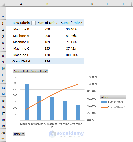
To Create A Pareto Chart, Start By Making A Pivot Table From Your Data Range.
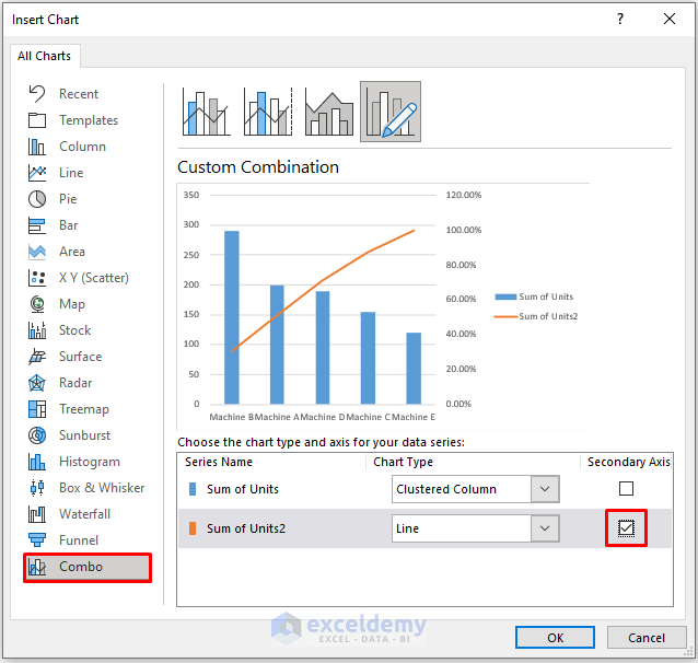
On the insert tab, in the charts group,. Select the entire data set (a1:c10), go to. Once your data is sorted and the cumulative percentage is calculated, you can create a pareto chart by. Here are the steps to create a pareto chart in excel:
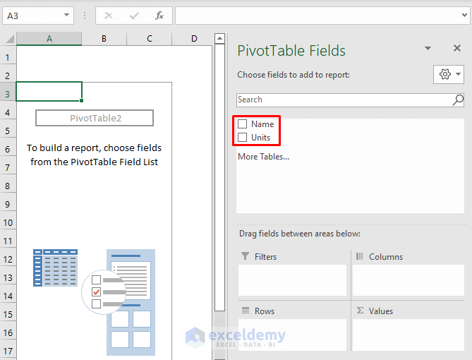
Set Up Your Data As Shown Below.
To create a pareto chart in excel 2016 or later, execute the following steps. In this article, we'll walk through the process of transforming a pivot table into a pareto chart. We'll explore why you'd want to use a. Select any data from your dataset.